Shape Functions for Concave Quadrilaterals

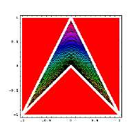
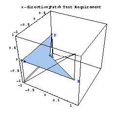
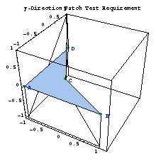
Continuous domains can be modeled using either the finite or boundary element methods. Both require test functions to be used as interpolants. A shape function can be viewed as a specific solution to an elliptic equation on a given polygonal domain. For convex n-sided polygons these functions can readily be found in closed form as rational polynomials. However, convexity is too restrictive a requirement for smooth modeling of many continuous domains. Examples include analysis of biological entities, soil-structure interaction, and high precision graphics rendering. The concavity restriction is alleviated by analytically enforcing continuity of the displacement, slope and curvature tensor fields. In particular, for the simplest concave shape, the four-noded element, the shape function associated with the concave node is calculated. The three remaining shape functions are generated using the three patch test requirements, which require reproducibility of any arbitrary linear field

Radiographic Images:

Diagnoses made from MRI, X-ray, CT-scan and other imaging techniques are based on the comparison of medically significant points and boundaries. In order to be able to consistently compare such images coordinate invariant shape analysis is necessary. In the case of the Maxillo-Facial frame nodal points are found from CT scans, these points form the outline of a concave shape. Apparently the concavity is essential to the proper growth and function and thus needs to be considered in comparative analysis. If the domain outlined by the nodes is discretized into convex parts then the concavity information is lost.

Earthquake Behavior Prediction:

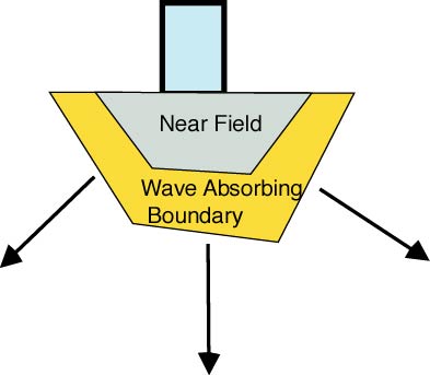
The prediction of earthquake's effect on the stability of buildings requires an efficient modeling of the soil structure interaction. Generally the ground is considered to be an semi-infinite domain since the soil is significantly larger than the building. The wave absorbing boundary is necessarily concave. If the boundary is discretized numerical modeling will predict that waves will pass between the arbitrary piece. The spurious waves cloud the solution related to the incoming and outgoing waves which pass through the wave absorbing boundary and are observed in in situ earthquake measurements.

3-D Representation:

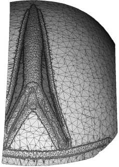
When an object is rendered it must first be discretized into two dimensional shapes depending on the viewing angle. Any discretization beyond adds more data to the image than is provided in the original shape. Commonly objects are rendered using a triangular domain discretization. The mesh division is not only time consuming, it is unnecessary if convex and concave shape functions can be found consistently in closed form.

Concave Shape:

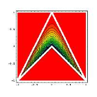
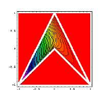
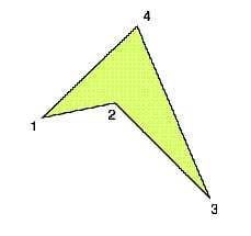
Here node-(2) is the concave node and the opposite concave node is node-(4). The elliptically condition dictates that the maximum and minimum values of all the shape functions must occur at the boundary. The lowest order shape functions are single valued at only one node and zero valued at all others. Along the boundary between the zero and single valued nodes the behavior is linear.

The Three Patch Test Requirements:

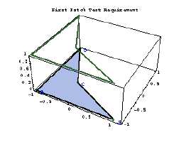
First Attempt, Isoparametric Formulation:

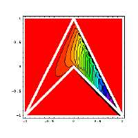
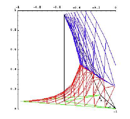
The first attempt at finding the shape functions along the boundary is applying the isoparametric formulation generally used for trapezoidal domains. Notice that while it is linear along the zero to one boundary and zero on all others the shape function is not contained in the concave domain. Also, the function bifurcates.